E4S

Project: Digital Signal Processing

In this project you will capture digital samples from the Electret microphone, display a waveform, then perform Fourier spectral analysis to measure the noise floor and identify the dominant frequency present. You will learn about and apply two digital signal processing techniques: downsampling and fast Fourier transforms (FFT).

Build the Circuit

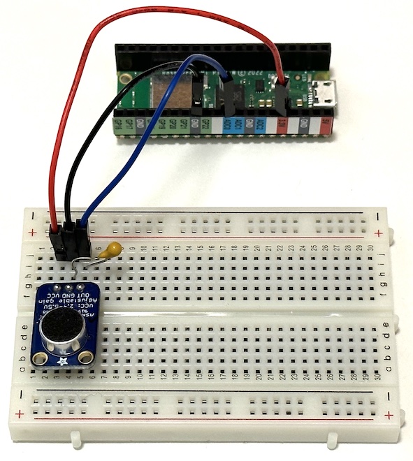
Power down your Pico then plug the Electret microphone into your breadboard and use jumper wires for make the following connections:

Mic Vcc to Pico 3.3V
Mic OUT to Pico ADC0
Mic GND to Pico GND

Finally, add a 1μF capacitor (the one with a “K”) to your breadboard between the Mic OUT and GND pins. This will filter out some of the high-frequency electronic noise that can contaminate the ADC measurement. Your completed circuit should look similar to this:

electret mic circuit

Start here for a brief introduction to electret microphones. The adafruit product page has more details on the board we are using.

Read Samples

Use the following program to digitize 512 samples of the microphone signal as fast as possible:

import time

import board
import analogio

NSAMPLES = 512

mic = analogio.AnalogIn(board.A0)

while True:
    time.sleep(1)
    start = time.monotonic_ns()
    samples = [mic.value for i in range(NSAMPLES)]
    stop = time.monotonic_ns()
    duration_ns = stop - start
    print(f'duration = {1e-6*duration_ns:.1f}ms')

Each sampling loop should have a duration of about 6ms. Add code to calculate and print the sampling rate in KHz, i.e. the average frequency at which each of the NSAMPLES samples are recorded. Call this sampling rate f0 in your code. How does your calculated value of f0 compare with the upper limit of typical human hearing? If you value of f0 is less than 10 KHz, check your calculation.

Plot Samples

Update your code to convert the samples in ADU to millivolts. Note that the Pico analog-to-digital converter resolution is only 12 bits but the 16-bit ADU values have 16-bit resolution, where 0xffff represents 3.3V. Therefore the appropriate conversion factor is 3300/0xffff mV/ADU.

Modify your code to print the first 100 mean-subtracted sample values so that the Mu Editor will display them in its Plotter window. Note that the Plotter window only displays about 100 points at a time, so printing more values to plot would only slow the program down without plotting any more data.

Note that the Plotter Window automatically scales its y axis so the plot amplitude can appear to suddenly change when the signal level crosses certain thresholds.

Even with no sound present, your plotted waveform might show some high-frequency “ripple”. If you observe this, check that the 1μF capacitor is doing its job by temporarily removing it. Verify that your waveform is centered on zero: if not, check that your code is correctly calculating and subtracting the mean measurement value.

Audio Test Setup

Use this online tone generator to play a continous 880 Hz sine wave through your laptop or phone speaker (you will need to change the frequency from the default 440 Hz). Adjust the position of your microphone relative to your laptop or phone speakers and the output volume until the Mu Editor plot clearly shows a single cycle of a sine wave. Be sure to protect your ears by using the lowest output volume possible and wearing ear plugs if necessary. You can also place your phone and breadboard close together under some sound insulation (jacket, blanket, etc).

You should aim for an sine-wave amplitude of about 1000 mV, i.e. 1 Volt, which will mostly be influenced by the relative positions of the speaker emitting the 800 Hz tone and your electret microphone. In case the amplitude of your waveform is still low after trying different positions, you may need to increase the amplification of the microphone circuit by turning the adjustment potentiometer screw shown below to its maximum counter-clockwise position:

electret amplification adjustment

Enhanced Resolution

Since we are able to read samples relatively fast compared with a typical audio frequency, we can afford to sacrifice some speed for accuracy. The easiest way to accomplish this is to average consecutive samples, which is a signal-processing technique known as “downsampling”.

Modify your code as follows:

NAVG = 8
NMEASURE = 512
NSAMPLES = NAVG * NMEASURE

then add code to downsample from NSAMPLES samples to NMEASURE averages. Call your array of averaged values measurements.

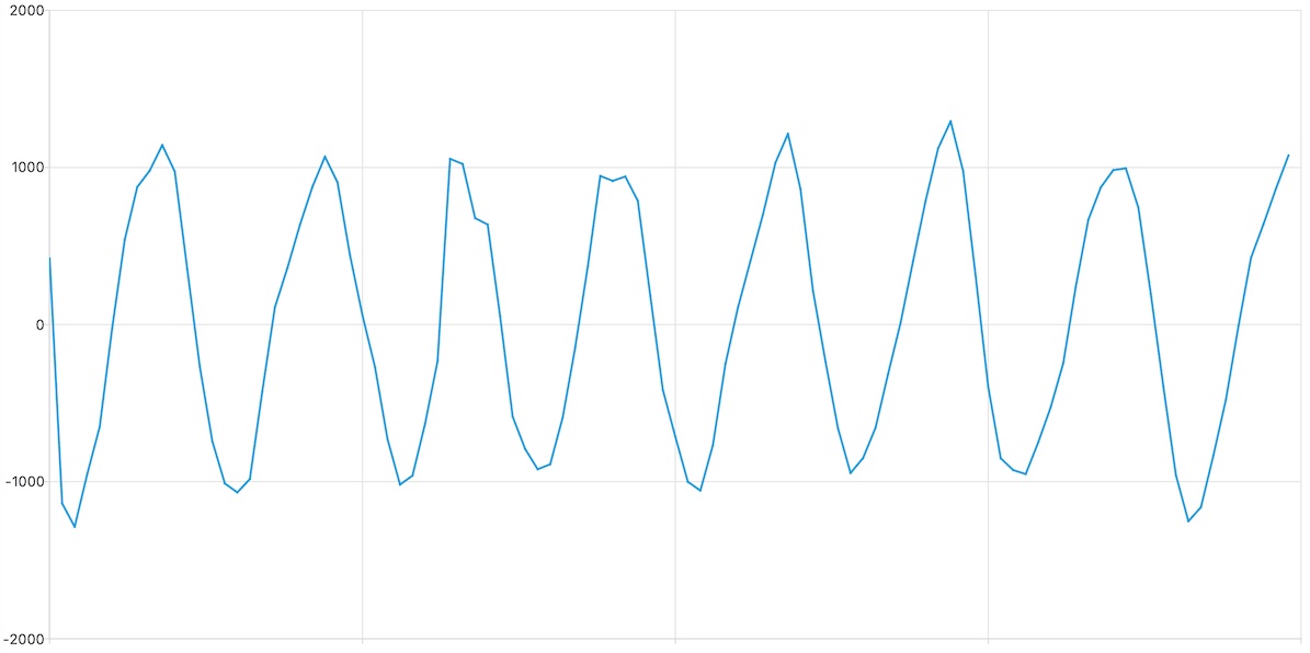
Plot the first 100 measurements and compare the new graph with the same audio test setup. If you did this correctly, the new graph should be compressed along the time axis (by a factor of NAVG) and have less noise (by a factor of sqrt(NAVG)). This digital signal processing method has effectively provided almost three extra bits of resolution, at the expense of 8x slower sampling.

Verify that, instead of 1 sine cycle, you now see about 8 cycles in your plot. Also, verify that you have about the same amplitude as before (otherwise, check the normalization of your average calculation). Your waveform should look similar to this:

800Hz tone waveform

Enter the Frequency Domain

We now want to estimate the frequency of the sine wave in our audio test setup. Our sequence of samples are in the “time domain”, where a sine wave has its familar shape. To identify the frequency of a periodic signal, it is convenient to work instead in the “frequency domain” where a sine wave is delta function at a location determined by its frequency. Both domains contain exactly the same amount of information and we can move back and forth using discrete Fourier transforms.

To perform a Fourier transform using the standard formulas requires on the order of NMEASURE**2 floating-point operations. However, there is a clever way of reorganizing the calculation known as the fast Fourier transform (FFT) which only requires on the order of NMEASURE * log(NMEASURE) operations. The FFT algorithm is implemented in the CircuitPython ulab library, which implements a subset of the popular numpy library. One restriction of the FFT algorithm is that the input array size must be a power of 2, which is why we chose 512 = 2**9 above. (If you ever need the fastest possible FFT algorithm, check out FFTW which also relaxes the power of two requirement).

Comment out your plotting loop (which will disable the Mu Editor plot display) and add the following code to calculate the Fourier transform of your averaged samples:

measurements = ulab.numpy.array(measurements)
fft_real, fft_imag = ulab.numpy.fft.fft(measurements)

The first line converts your python list of measurement values to the ulab internal array format, which is more efficient than a python list when all elements have the same data type. The second line calculates the FFT and returns two arrays that represent the real and imaginary parts of the complex-valued result. You will also need to

import ulab

near the top of your code, in order to use any of the ulab library routines.

Why is the FFT result complex valued? This seems to indicate that there is more information in the frequency domain, since we have twice as many array elements, which contradicts what we claimed earlier. However, there is a symmetry that ensures information is conserved,

(fft_real[i] == +fft_real[NMEASURE - i]) and (fft_imag[i] == -fft_imag[NMEASURE - i])

for 0 < i < NMEASURE/2. Print a few values to convince yourself that this is true (it might not be true exactly, because of round-off errors, but should be very close). Because of this symmetry, all of the information in FFT is contained within the first half of the array i < NMEASURE/2. (Technically, the values with i > NMEASURE/2 correspond to negative frequencies.)

Although we will not use it in this project, a simple modification of the FFT, known as the “inverse FFT”, transforms from the frequency domain back to the time domain. Both transforms generally expect a complex-valued input and return a complex-valued result but, when the input is real (or imaginary), the result will have a symmetry that conserves information and ensures that the reverse transform is real (or imaginary).

Power Play

You can think of the FFT as a recipe for building the time domain signal as a sum of sines and cosines at specific frequencies f[i] = i * df, where df = f0 / (NMEASURE * NAVG), with amplitudes related to fft_real[i] and fft_imag[i] (for i < NMEASURE/2). The zero frequency value corresponds to a constant (in time) value, also known as the “DC component”. Since we subtracted off the mean earlier, this should be zero and we will ignore it. (In fact, it will not be exactly zero because of round-off errors in the calculation and subtraction of the mean.)

Since we do not care about the phase differences (sine vs cosine) at each frequency, we will combine the real and imaginary FFT values into their complex magnitude squared, scaled by the number of measurements. One way to accomplish this would be with a loop:

for i in range(NMEASURE):
    power[i] = (fft_real[i] ** 2 + fft_imag[i] ** 2) / NMEASURE

However, a nice feature of ulab (and numpy) is that you can write a formula that applies to all elements of an array without any explicit loop as:

power = (fft_real ** 2 + fft_imag ** 2) / NMEASURE

The resulting power is an array, not a single number! This trick is known as vectorization and leads to code that is easier to read and often much faster.

These magnitude squared FFT values are referred to as “power” since they are related to electrical power when the time-domain consists of voltage measurements (but the power terminology is often also used for non-voltage measurements).

Noise Level

Estimate the amount of noise in your measurements with two different methods, one in the time domain and other in the frequency domain:

noise_time = ulab.numpy.std(measurements) ** 2
noise_freq = ulab.numpy.mean(power[1:NMEASURE//2])

Calculate and print the results of both of these methods when your setup is relatively quiet. Notice how similar they are! This is another demonstration that the two domains contain equivalent information, and a consequence of Parseval’s theorem.

The first method calculates the variance of your averaged time-domain samples, i.e. the squared width of a histogram of the samples. The second method calculates the average power over all (positive) frequencies, i.e. excluding the i=0 DC component and and the i >= NMEASURE/2 (negative) frequencies that are redundant by symmetry.

Observe typical noise levels when your environment is quiet, then add a line near the top of your program to record the typical level:

NOISE_LEVEL = ...

Note that the units of power and this noise measurement are mV-squared.

Frequency Measurement

Now that you have established the typical noise level of your audio environment, you are ready to identify a signal with a dominant frequency that is significantly above the noise level.

Modify your code to loop over the power values for 1 <= i < NMEASURE // 2 and find the largest value. If this is at least 100 times larger than your NOISE_LEVEL, then print the corresponding frequency in Hertz, i * df, with df defined above (but note that df will be in KHz if f0 is in KHz).

Test your frequency measurement program with the reference 1600 Hz tone. What is the frequency resolution of your measurement, i.e. what is the smallest difference in frequency that you can detect? Is your measurement consistent with the known value of 1600 Hz given this resolution? Is this resolution sufficient for a musical instrument tuner?

Try varying the tone frequency over the range 400 - 3200 Hz (3 octaves) and see how accurately you are able to measure different frequencies. You may need to increase the volume at lower frequencies in order to reach the 100x noise detection threshold.

This site is open source. Improve this page.